Summary
In this post, I train LeWM without SIGReg and compare its embeddings with normal runs.
Q: What’s the purpose of this experiment?
I want to see what SIGReg does. To do this, I compare the embeddings of models trained with and without SIGReg, and look for representation collapse in the model without it.
The non-SIGReg models is trained with the same setup as my baseline (image size 112, 3 epochs), except that the SIGReg weight ($\lambda) is set to 0.
In addition, I also look at the embeddings of another model trained with image size 224 and 3 epochs.
Q: What types of collapse am I looking for?
- Complete collapse. All images map to almost the same point and the spread becomes very small.
- Dimensional collapse. The points spread out, but only along a few directions. The other directions are not used.
Q: What is the input data?
I created a script that encodes a fixed set of frames with each checkpoint and saves the embeddings (cls, emb) and the true state and proprio of each frame.
I use all 3 checkpoints from each of these runs:
- pusht/2026-09-28_114752_img112_s3072 (image size 112, 3 epochs)
- pusht/2026-10-14_115337_img112_s3072_nosigreg (same as above but without SIGReg)
and all 10 checkpoints from:
- pusht/2026-10-10_120411_img224_s3072 (image size 224, 10 epochs)
The frames are in two groups: 20,000 random frames from the whole dataset, which I use for the statistics, and 1,094 frames of 10 random episodes, which I use to draw trajectories in the PCA plots. That is 21,094 frames in total.
Q: For each test, what metrics are compared?
- Scale: how big is the point cloud.
- length of mean vector (|mean|)
- spread
- spread / |mean|
- Direction: are all the points in the same directions?
- histogram of 1 - cosine similarity
- calculated between random frames
- Eigenvalue spectrum: how many directions are used?
- eigenvalues of covariance matrix
- effective rank
- participation ratio
- Is the distribution close to N(0,I)?
- SIGReg statistic
- histogram along random directions
- Linear probe
- train a ridge regression from latent to states (agent x, agent y, block x, block y, cos(block angle), sin(block angle))
- PCA
- does any principal component match the position or angle of the T block?
Q: What does the result say? What’s the restriction or drawback of SIGReg?
Without SIGReg, the embeddings collapse completely: the spread is about 10⁻⁵, compared with about 14 with SIGReg. The planner cannot use this model: its success rate on PushT is only 2.8% (mean of 5 seeds).
With SIGReg, there is no complete collapse, but there is some dimensional collapse: the effective rank is only about 69 of 192 at epoch 3.
Longer training moves the distribution closer to N(0, I), but it does not get very close. In the 10-epoch run, the effective rank stops at about 98. (This run also uses a larger image size, so the comparison is not clean.)
Q: Future experiments I want to run?
The PushT scene has only about 5 degrees of freedom, but the latent has 192 dimensions. This can limit how many dimensions the encoder can use. A more complex scene may show if this is the cause.
Experiment Details
All results are from the notebook playground/sigreg_collapse_notebook.py in the le-wm repo. Unless I say otherwise, the latent is emb (the projector output, which is the input of the predictor and the latent that SIGReg acts on), and the epoch is 3, the last epoch that all three runs have.
| Run | SIGReg weight | Image size | Epochs | Folder |
|---|---|---|---|---|
| SIGReg (baseline) | 0.09 | 112 | 3 | pusht/2026-09-28_114752_img112_s3072 |
| no SIGReg | 0 | 112 | 3 | pusht/2026-10-14_115337_img112_s3072_nosigreg |
| SIGReg 10 epochs (img224) | 0.09 | 224 | 10 | pusht/2026-10-10_120411_img224_s3072 |
Summary table
emb, epoch 3:
| Measure | SIGReg | no SIGReg | SIGReg 10 epochs (img224) |
|---|---|---|---|
| spread () | 13.9 | 1.2 × 10⁻⁵ | 13.9 |
| |mean| | 0.39 | 0.16 | 0.67 |
| effective rank (max 192) | 69.4 | 29.2 | 78.6 |
| participation ratio | 64.4 | 15.1 | 74.2 |
| directions for 99% of variance | 74 | 86 | 79 |
| SIGReg statistic, raw (N(0, I): 1.05) | 1.50 | 51.5 | 1.55 |
| SIGReg statistic, standardized | 1.46 | 2.90 | 1.40 |
| mean linear probe R² | 0.85 | 0.54 | 0.96 |
1. Scale: how big is the point cloud?
- |mean|: the length of the mean latent vector, i.e. the position of the center of the cloud.
- spread: the square root of the total variance (the sum of the variances of all 192 dimensions). It is the typical distance from a point to the center. For N(0, I) in 192 dimensions, the spread is .
- spread / |mean|: the size of the cloud relative to its distance from 0. A very small value means that all points are at almost the same place, far from 0.
| Run | Epoch | |mean| | spread | spread / |mean| | smallest dim std | largest dim std |
|---|---|---|---|---|---|---|
| SIGReg | 1 | 1.22 | 13.7 | 11.2 | 0.79 | 1.19 |
| SIGReg | 2 | 0.61 | 13.9 | 22.7 | 0.81 | 1.17 |
| SIGReg | 3 | 0.39 | 13.9 | 35.6 | 0.81 | 1.17 |
| no SIGReg | 1 | 0.20 | 2.0 × 10⁻⁴ | 1.0 × 10⁻³ | 4.6 × 10⁻⁶ | 4.5 × 10⁻⁵ |
| no SIGReg | 2 | 0.16 | 3.6 × 10⁻⁵ | 2.2 × 10⁻⁴ | 1.7 × 10⁻⁶ | 4.1 × 10⁻⁶ |
| no SIGReg | 3 | 0.16 | 1.2 × 10⁻⁵ | 7.3 × 10⁻⁵ | 5.5 × 10⁻⁷ | 1.4 × 10⁻⁶ |
| SIGReg 10 epochs (img224) | 3 | 0.67 | 13.9 | 20.9 | 0.81 | 1.19 |
| SIGReg 10 epochs (img224) | 10 | 0.35 | 13.8 | 39.9 | 0.82 | 1.15 |
The plot below shows the std of each of the 192 dimensions, sorted from the largest to the smallest. The y-axis is logarithmic.
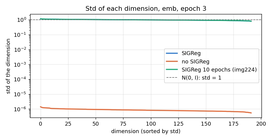
Std of each dimension of emb at epoch 3. The SIGReg runs stay near 1. The no-SIGReg run is about 10⁶ times smaller in every dimension.
Result. Without SIGReg, the cloud is complete collapse: the spread is 1.2 × 10⁻⁵, and it becomes smaller at each epoch (2.0 × 10⁻⁴ → 3.6 × 10⁻⁵ → 1.2 × 10⁻⁵). With SIGReg, every dimension has a std between 0.8 and 1.2, and the spread is very close to .
2. Direction: are all points in the same direction?
I take 5,000 random pairs of frames and calculate the cosine similarity of their latents. The plot shows 1 − cosine similarity on a log x-axis. For N(0, I), two random vectors are almost perpendicular, so 1 − cos is near 1. If the latents collapsed, all pairs point in the same direction, and 1 − cos is near 0.
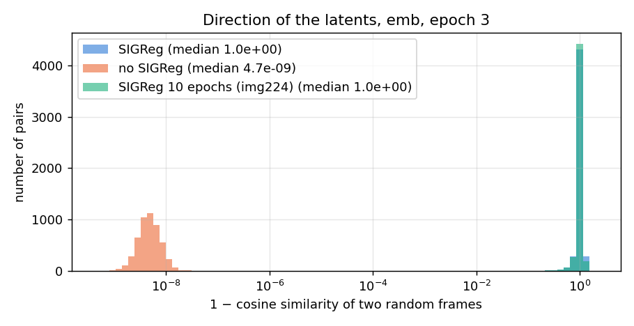
1 − cosine similarity of random pairs of frames, emb, epoch 3.
Result. The median of 1 − cos is 1.01 for SIGReg, 1.02 for the img224 run, and 4.7 × 10⁻⁹ for no SIGReg. Without SIGReg, all latents point in the same direction (the cloud is a very small ball at distance 0.16 from 0).
3. Eigenvalue spectrum: how many directions are used?
The eigenvalues of the covariance matrix are the variances along the principal components. The left plot shows the raw eigenvalues (for N(0, I), all are 1). The right plot divides them by their sum, so it shows only the shape of the cloud.
Two numbers summarize the shape:
- Effective rank: the exponential of the entropy of the normalized eigenvalues:
- Participation ratio: . It gives more weight to the large eigenvalues.
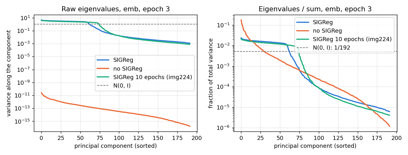
Eigenvalue spectrum of emb at epoch 3. Left: raw eigenvalues. Right: eigenvalues divided by their sum.
| Run | Epoch | Effective rank | Participation ratio | Top component share | Directions for 90% | Directions for 99% |
|---|---|---|---|---|---|---|
| SIGReg | 1 | 55.0 | 49.9 | 2.9% | 44 | 61 |
| SIGReg | 2 | 67.0 | 61.8 | 2.5% | 55 | 72 |
| SIGReg | 3 | 69.4 | 64.4 | 2.3% | 56 | 74 |
| no SIGReg | 1 | 21.2 | 11.9 | 19.6% | 22 | 61 |
| no SIGReg | 2 | 27.6 | 13.9 | 18.1% | 32 | 86 |
| no SIGReg | 3 | 29.2 | 15.1 | 17.4% | 32 | 86 |
| SIGReg 10 epochs (img224) | 3 | 78.6 | 74.2 | 2.1% | 66 | 79 |
| SIGReg 10 epochs (img224) | 10 | 97.8 | 93.6 | 1.7% | 83 | 97 |
Result: SIGReg runs have a dimensional collapse.
- There is a “cliff”. In the right plot, the SIGReg run drops near component 60, and the img224 run drops near component 75. At the cliff, the values fall by about 100 times. After the cliff, each direction has only 10⁻³ to 10⁻⁵ of the total variance, which is 5 to 500 times less than an equal share (1/192 ≈ 5 × 10⁻³).
- The used directions are larger than in N(0, I). In the left plot, the first 60–75 eigenvalues are about 2–4. SIGReg keeps the std of each coordinate near 1, so the total variance stays near 192. But only about 65 directions share it, so each gets about 192 / 65 ≈ 3. The cloud is a flat “pancake”: wide in about 65 directions and very thin in the others.
| Run (epoch 3) | Share of components 1–60 | Share of components 76–192 | Mean eigenvalue, 1–60 | Mean eigenvalue, 76–192 |
|---|---|---|---|---|
| SIGReg | 94.7% | 0.86% | 3.04 | 0.014 |
| no SIGReg | 97.1% | 1.53% | 2.3 × 10⁻¹² | 1.9 × 10⁻¹⁴ |
| SIGReg 10 epochs (img224) | 84.2% | 1.88% | 2.71 | 0.031 |
The no-SIGReg line in the right plot has no meaning. It looks “normal”: it decreases slowly, with no cliff. But the left plot shows that its eigenvalues are only 10⁻¹¹ to 10⁻¹⁶, so the cloud is almost one point. The right plot removes the size, so the shape of this tiny cloud tells nothing. For the same reason, its “directions for 99%” (86) is higher than for the SIGReg run, but this is not a good sign.
4. Is the distribution close to N(0, I)?
4.1 The SIGReg statistic
I calculate the SIGReg loss as in training: random batches of 128 frames, 1024 random directions, averaged over the batches. All models use the same batches and directions (fixed seed).
The batches must be random. The frames in the files are sorted by dataset row, and nearby episodes look alike. A first version without the shuffle gave about 14 for the SIGReg run at epoch 3, compared with 1.5 with random batches.
The value is about , where is a noise floor (a finite batch is never exactly Gaussian), is the batch size, and is the real distance from N(0, I). Real samples from N(0, I) give 1.05. Only the part above this floor is a real distance.
- Raw: on the latents as they are. This is what the training loss sees.
- Standardized: after each dimension is shifted and scaled to mean 0 and std 1. This removes the scale problem and shows only the shape problem.
| Run | Epoch | SIGReg (raw) | SIGReg (standardized) |
|---|---|---|---|
| SIGReg | 1 | 2.11 | 1.65 |
| SIGReg | 2 | 1.58 | 1.49 |
| SIGReg | 3 | 1.50 | 1.46 |
| no SIGReg | 1–3 | 51.5 | 3.13 → 2.90 |
| SIGReg 10 epochs (img224) | 3 | 1.55 | 1.40 |
| SIGReg 10 epochs (img224) | 10 | 1.33 | 1.29 |
| N(0, I) reference | 1.05 | 1.05 |
4.2 Histograms along random directions
I take 4 random unit directions (the same for all runs) and project every latent on them. The gray curve is the N(0, 1) density. All plots use the same x-axis (−4 to 4), so that a collapsed cloud shows as one thin spike and is not stretched to look like a bell curve.
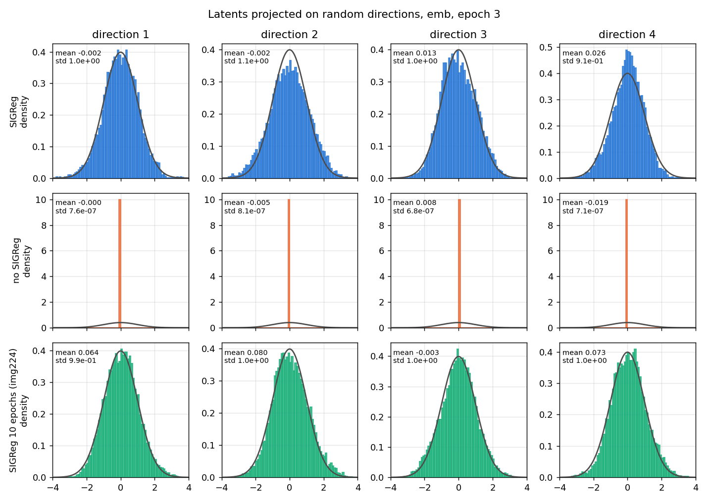
emb at epoch 3, projected on 4 random directions. The text in each plot gives the real mean and std of the projected values.
Result. The SIGReg runs follow the gray curve well. For no SIGReg, all values fall into one bar (its height is 10, because the bar is 0.1 wide and holds all the frames).
5. Linear probe: is the information about the scene still there?
I fit a ridge regression from the standardized latent to the true state: agent x, agent y, block x, block y, cos(block angle), sin(block angle). Train and test frames come from different episodes (80% / 20%). Because the latent is standardized first, the probe does not see the scale, so even a cloud that is 10⁻⁵ wide can give a good result.
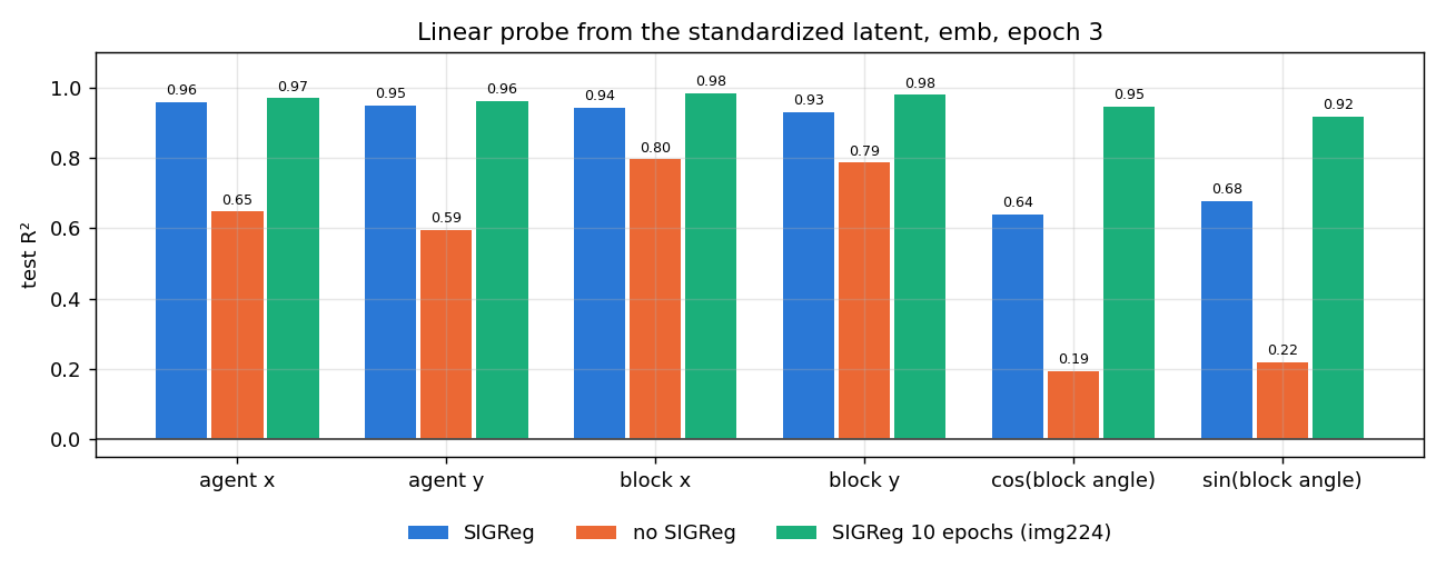
Test R² of the linear probe from standardized emb, epoch 3.
| Run (epoch 3) | agent x | agent y | block x | block y | cos(angle) | sin(angle) | mean |
|---|---|---|---|---|---|---|---|
| SIGReg | 0.96 | 0.95 | 0.94 | 0.93 | 0.64 | 0.68 | 0.85 |
| no SIGReg | 0.65 | 0.59 | 0.80 | 0.79 | 0.19 | 0.22 | 0.54 |
| SIGReg 10 epochs (img224) | 0.97 | 0.96 | 0.98 | 0.98 | 0.95 | 0.92 | 0.96 |
Result. The collapsed latent still has some information about the positions, but much less about the block angle. The probe R² of no SIGReg does not change from epoch 1 to 3 (0.54). For the planner, this information is not useful: the planner compares raw latents with a squared distance, and when all distances are about 10⁻¹⁰, the cost differences between action plans are almost 0.
The block angle is the hardest target for the 3-epoch SIGReg run (R² ≈ 0.65). The img224 run learns it much better (0.92–0.95 at epoch 3).
6. PCA
For each run, I fit a PCA on the 20,000 random frames and plot PC1 against PC2. The colors are the true state (the model never sees it): block angle in the top row, agent x in the bottom row. The black lines are 3 full episodes, with frames connected in time order.
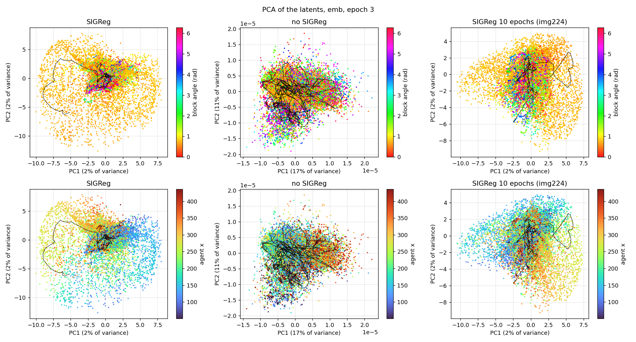
PCA of emb at epoch 3. Top: colored by block angle. Bottom: colored by agent x. Black lines: 3 episodes. Each plot has its own axes.
| SIGReg | no SIGReg | SIGReg 10 epochs (img224) | |
|---|---|---|---|
| Size of the cloud | normal (about ±10) | about 10⁻⁵ (complete collapse) | normal (about ±8) |
| Variance in PC1 + PC2 | 4% | 28% | 4% |
| Agent x colors | clear change from left (large x) to right (small x) | small change from left to right | clear pattern |
| Angle colors | outer frames almost all orange (about 0.8 rad), center mixed | mixed | same as SIGReg |
| Black lines | smooth, with one large loop | long jumps in a tangle | mostly smooth |
- Size. The no-SIGReg cloud is about 10⁶ times smaller than the other two. The three plots look the same size only because each has its own axes.
- Share of variance. In the SIGReg runs, about 65 directions share the variance, so each PC has only about 2%, and the plot shows only about 4% of the cloud.
- Orange outer frames. Many frames have a block angle near 0.8 rad. This is possibly the goal angle of PushT, π/4 ≈ 0.785. I did not verify this.
- No PC matches one state. A PC is a mix of several states, so the patterns are rough. Agent x shows the clearest pattern. The block angle shows no clear pattern in PC1–PC2.
7. Change over epochs
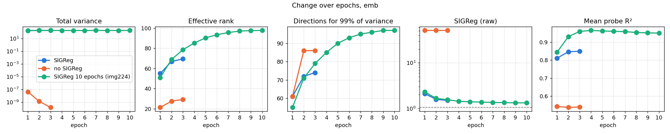
Main metrics of emb at every epoch. Dashed line in the SIGReg panel: N(0, I) reference.
- No SIGReg collapses already at epoch 1 (total variance 4 × 10⁻⁸), and it becomes smaller at each epoch. A checkpoint is saved only at the end of each epoch, so I cannot see when the collapse starts inside epoch 1.
- SIGReg: the effective rank goes up from 55 to 69 in 3 epochs.
- SIGReg 10 epochs (img224): the total variance is constant at about 192. The effective rank goes up from 51 (epoch 1) to 98 (epoch 10), and it stops at about epoch 8.
| Epoch | Spread | Effective rank | Participation ratio | Directions for 99% | SIGReg (raw) | Mean probe R² |
|---|---|---|---|---|---|---|
| 1 | 13.7 | 50.9 | 46.2 | 55 | 2.31 | 0.843 |
| 2 | 13.9 | 68.9 | 64.1 | 71 | 1.66 | 0.930 |
| 3 | 13.9 | 78.6 | 74.2 | 79 | 1.55 | 0.959 |
| 4 | 13.8 | 85.2 | 80.6 | 85 | 1.44 | 0.965 |
| 5 | 13.8 | 90.4 | 85.9 | 90 | 1.40 | 0.962 |
| 6 | 13.8 | 93.4 | 89.0 | 93 | 1.38 | 0.960 |
| 7 | 13.9 | 95.6 | 91.3 | 95 | 1.35 | 0.958 |
| 8 | 13.8 | 97.1 | 92.9 | 96 | 1.34 | 0.953 |
| 9 | 13.8 | 97.6 | 93.4 | 97 | 1.33 | 0.951 |
| 10 | 13.8 | 97.8 | 93.6 | 97 | 1.33 | 0.950 |
The SIGReg statistic goes down while the rank goes up (2.31 → 1.33), so the SIGReg loss “sees” the low rank and pushes against it. At epoch 10, the part above the N(0, I) floor is only about 0.3.
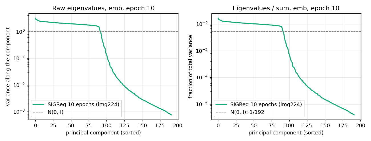
Eigenvalue spectrum of emb for the img224 run at epoch 10. The cliff moved to about component 90, but about half of the 192 directions are still almost unused.
Why the rank does not go higher. A separate test on the SIGReg run at epoch 3 whitened the latents (it made all eigenvalues equal to 1 and kept the rest of the shape). This removed about 90% of the distance above the floor. So most of the remaining SIGReg loss comes from this anisotropy. But with a batch size of 128, it adds only about 0.45 to the loss, which is less than the noise floor (about 1.05). So the signal against the remaining anisotropy is weak. A larger batch or a larger SIGReg weight makes this signal stronger.
Be careful with these comparisons:
- Learning-rate schedule. The scheduler is a linear warmup and a cosine decay to 0 over all training steps. In the 3-epoch run, the learning rate is almost 0 at the end of epoch 3. In the 10-epoch run, it is still about 80% of the peak at the end of epoch 3. This is one reason why the 3-epoch run stops at about 69. It also means that the plateau at epochs 8–10 can come from the learning rate that goes to 0, and not from a real limit.
- Image size. The 10-epoch run uses 224-pixel images, and the baseline uses 112. The image size and the training length change together.
- One seed. Each run is one training run.
8. The encoder output (cls)
The projector is Linear → BatchNorm → GELU → Linear, so the BatchNorm is in the hidden layer and does not prevent a collapse of emb. To see if the encoder itself collapsed, I also look at cls (the encoder CLS token, before the projector).
| Run (epoch 3) | |mean| | spread | effective rank | SIGReg (raw) | mean probe R² |
|---|---|---|---|---|---|
| SIGReg | 6.94 | 12.0 | 30.8 | 19.8 | 0.87 |
| no SIGReg | 13.6 | 1.6 × 10⁻⁴ | 37.2 | 130 | 0.55 |
| SIGReg 10 epochs (img224) | 7.16 | 11.8 | 26.1 | 20.6 | 0.97 |
- Without SIGReg, the encoder output also collapses completely (spread 1.6 × 10⁻⁴ at a distance of 13.6 from 0). So the collapse is not only in the projector.
- With SIGReg,
clsis not collapsed, but its effective rank is much lower thanemb(31 vs 69 at epoch 3; 36 vs 98 at epoch 10 for the img224 run). SIGReg acts onemb, not oncls, so the projector spreads a lower-rank encoder output over more directions.
9. Planning success rate
I evaluated the no-SIGReg model (epoch 3) with the CEM planner on PushT, with 5 different seeds. Each seed gives a different set of 50 start states from the dataset. The goal is the expert’s state 25 steps later, and the planner has 50 steps to reach it.
python eval.py --config-name=pusht.yaml policy=pusht/2026-10-14_115337_img112_s3072_nosigreg/weights_epoch_003.pt eval.img_size=112 seed=<0..4>
| Seed | Success rate |
|---|---|
| 0 | 2.0% |
| 1 | 4.0% |
| 2 | 0.0% |
| 3 | 4.0% |
| 4 | 4.0% |
| Mean ± std | 2.8% ± 1.8% |
Result. The planner reaches the goal in only 0–2 of 50 episodes for each seed. This agrees with section 5: when all latents are at almost the same point, the planning cost is almost the same for all action plans, so the planner cannot select a good plan.
I did not evaluate the SIGReg baseline or a random policy with the same seeds yet, so I cannot say if 2.8% is better than chance.